Shinnar-Le Roux Pulses

This page illustrates Shinnar-Le Roux (SLR) pulse design for MRI using the Julia package MRIPulses.

This page comes from a single Julia file: slr.jl.

You can access the source code for such Julia documentation using the 'Edit on GitHub' link in the top right. You can view the corresponding notebook in nbviewer here: slr.ipynb, or open it in binder here: slr.ipynb.

Setup

First we add the Julia packages that are need for this demo. Change false to true in the following code block if you are using any of the following packages for the first time.

if false
    import Pkg
    Pkg.add([
        "BlochSim"
        "InteractiveUtils"
        "LaTeXStrings"
        "LinearAlgebra"
        "MIRTjim"
        "MRIPulses"
        "Plots"
    ])
end

Tell this Julia session to use the following packages for this example. Run Pkg.add() in the preceding code block first, if needed.

using BlochSim: Spin, Position, signal, RF
using BlochSim: rf_slice, b1_gauss, rf_gauss
using BlochSim: excite!, spoil!, duration
using LaTeXStrings
using MRIPulses: dzrf
using MIRTjim: jim, prompt
using Plots: default, plot, plot!

default(titlefontsize = 10, markerstrokecolor = :auto, label="", width = 1.5)

WARNING: Imported binding BlochSim.rf_gauss was undeclared at import time during import to Main.

The following line is helpful when running this file as a script; this way it will prompt user to hit a key after each figure is displayed.

isinteractive() ? jim(:prompt, true) : prompt(:draw);

Baseline sinc pulse

tRF_ms = 1
n = 2^8 # how many samples
Δt_ms = tRF_ms / n # 3.90625 μs
nlobe = 3
α_deg = 60 # flip angle ° (somewhat large for testing)
α_rad = deg2rad(α_deg)
slice_width = 0.5 # cm
rf0, rephasing0 = rf_slice(tRF_ms ; nlobe, α_rad, Δt_ms, slice_width)
pulse0 = real(@. rf0.α * cis(rf0.θ)) # radians
label0 = "Sinc nlobe=$nlobe";

SLR pulse(s)

tb = 2nlobe # time-bandwidth
d1, d2 = 0.01, 0.01 # δ₁, δ₂ ripple design parameters
if 0 < α_rad < π/2 # use small tip :st and scale by flip angle
    ptype = :st; factor = α_rad
elseif π/2 ≤ α_rad < π # use :ex and scale up
    ptype = :ex; factor = α_rad/(π/2)
else
    error("unsupported flip $α_deg")
end
ftype1 = :pm
ftype2 = :ls
cancel_alpha_phs = false

pulse1 = dzrf(; n, tb, ptype, ftype=ftype1, d1, d2, cancel_alpha_phs)
@assert pulse1 ≈ real(pulse1)
pulse1 = factor * real(pulse1)
label1 = "SLR $ptype $ftype1"

pulse2 = dzrf(; n, tb, ptype, ftype=ftype2, d1, d2, cancel_alpha_phs)
@assert pulse2 ≈ real(pulse2)
pulse2 = factor * real(pulse2)
label2 = "SLR $ptype $ftype2" ;

Plot pulses

t = ((0:(n-1)) / n .- 0.5) * tRF_ms # [-tRF_ms/2, tRF_ms/2)
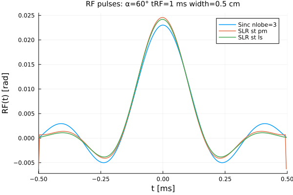
prf = plot(t, [pulse0 pulse1 pulse2],
  label = [label0 label1 label2],
  xaxis = ("t [ms]", (-1,1) .* (tRF_ms/2), ),
  yaxis = ("RF(t) [rad]", ),
  title = "RF pulses: α=$(α_deg)° tRF=$tRF_ms ms width=$slice_width cm",
)

prompt()

RF waveforms

Use the rephasing gradient from rf0. The rephasing gradient amplitude could be adjusted to better flatten the phase.

wave1 = pulse1 * b1_gauss(1, Δt_ms) # convert to Gauss for RF()
wave2 = pulse2 * b1_gauss(1, Δt_ms)
rf1 = RF(wave1, Δt_ms, 0, rf0.grad)
rf2 = RF(wave2, Δt_ms, 0, rf0.grad);

Array of spins

For a range of z-positions to examine slice profile

Mz0, T1_ms, T2_ms, Δf_Hz = 1, 400, 80, 9 # tissue parameters
zpos = range(-1, 1, 201) # z positions (cm)
zfov = only(diff([extrema(zpos)...])) # 2 cm

make_spins(Mz0, T1_ms, T2_ms, Δf_Hz) = map(zpos) do z
    pos = Position(0, 0, z)
    Spin(Mz0, T1_ms, T2_ms, Δf_Hz, pos)
end;

Excite and rephase the spins

function exciter(rf;
    T2_ms::Real = T2_ms,
    spins = make_spins(Mz0, T1_ms, T2_ms, Δf_Hz),
    rephasing = rephasing0,
    revert0::Bool = false, # revert signal back to center of RF pulse?
)
    map(spins) do spin
        excite!(spin, rf)
        spoil!(spin, rephasing)
    end;
    signal_out = signal.(spins)
    if revert0
        time_back_ms = duration(rf)/2 + rephasing.Tg
        signal_out .*= exp(time_back_ms / T2_ms) * # un-decay
            cis(2π * (time_back_ms/1000) * Δf_Hz) # un-precess
    end
    return spins, signal_out
end

spins0, signal0 = exciter(rf0)
spins1, signal1 = exciter(rf1)
spins2, signal2 = exciter(rf2);

Plot slice profiles

function plot_profile(spins, plabel; α_deg = α_deg,
    ymin = -0.2,
    ytick = ([0, cos(α_rad), sin(α_rad), 1],
        ["0", "cos($(α_deg)°)", "sin($(α_deg)°)", 1]),
)
    mx = map(spin -> spin.M.x, spins)
    my = map(spin -> spin.M.y, spins)
    mz = map(spin -> spin.M.z, spins)
    mmag = @. sqrt(mx^2 + my^2)
    mpha = @. atan(my, mx)

    xaxis = ("z [cm]", (-1,1), [-1, -slice_width/2, 0, slice_width/2, 1])
    pmag = plot(; xaxis, yaxis = ("", (ymin,1), ytick), legend = :right)
    plot!(zpos, mx, label = "Mx")
    plot!(zpos, my, label = "My")
    plot!(zpos, mz, label = "Mz")
    plot!(zpos, mmag, label = "|Mxy|")

    ppha = plot(; xaxis, legend = :right)
    plot!(zpos, mpha, label = "∠Mxy")

    return plot(pmag, ppha; layout = (2,1),
      plot_title = "Slice profile: $plabel, α=$(α_deg)° T2=$T2_ms ms",
    )
end;

pp0 = plot_profile(spins0, label0)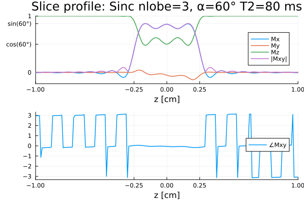

prompt()

pp1 = plot_profile(spins1, label1)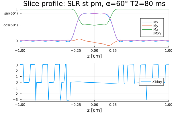

prompt()

pp2 = plot_profile(spins2, label2)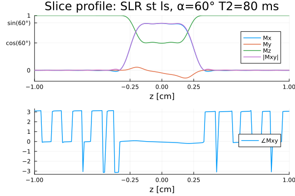

prompt()

Compare slice profiles

function plot_profile2(signals, labels;
    title = latexstring("|M_{xy}| \\ \\mathrm{and} \\ M_y \\ \\mathrm{ for } \\ α=$(α_deg)° \\ T_2=$T2_ms \\ \\mathrm{ms}"),
)
    xaxis = ("z [cm]", (-1,1), [-1, -slice_width/2, 0, slice_width/2, 1])
    ytick = ([0, sin(α_rad), 1], ["0", "sin($(α_deg)°)", 1])
    plot(; title, xaxis, yaxis = ("", (-0.2,1), ytick), legend = :right)
    plot!(zpos, abs.(signals); label=labels)
    plot!(zpos, imag.(signals); color=(1:3)')
end

signals = [signal0 signal1 signal2]
labels = [label0 label1 label2]
pmag1 = plot_profile2(signals, labels)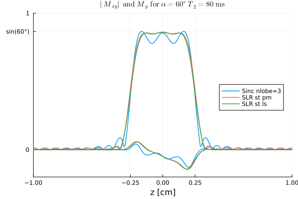

prompt()

Short T2 case

Here the profile is even farther from the target, even for a 0.5 ms RF pulse.

Seems like the "apparent" M₀ could be quite different for short T2 and long T2 spins, which could bias $f_{\mathrm{f}}$ in some types of scans.

T2_ms = 10
spins0, signal0 = exciter(rf0; T2_ms)
spins1, signal1 = exciter(rf1; T2_ms)
spins2, signal2 = exciter(rf2; T2_ms)
pmag2 = plot_profile2([signal0 signal1 signal2], labels)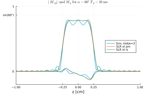

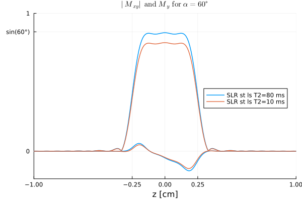
prompt()

Plot profiles at end of the rephasing gradient for two T2 values

T2 = [80, 10]
_, signal2a = exciter(rf2; T2_ms = T2[1], revert0 = false)
_, signal2b = exciter(rf2; T2_ms = T2[2], revert0 = false)
labels = [label2 * " T2=$t ms" for t in T2']
pmag3 = plot_profile2([signal2a signal2b], labels; title =
 latexstring("|M_{xy}| \\ \\mathrm{and} \\ M_y \\ \\mathrm{ for } \\ α=$(α_deg)°"),
)

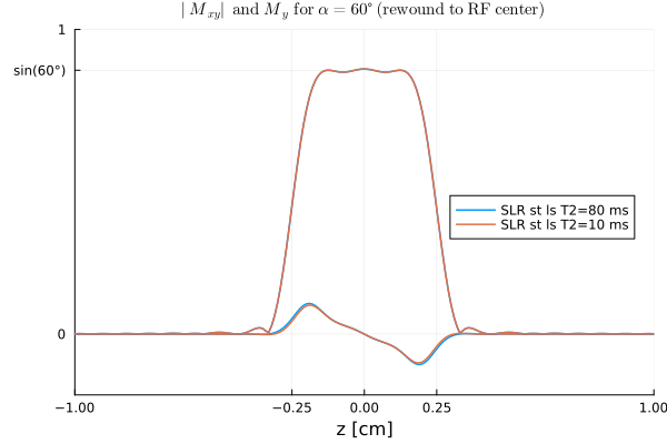
prompt()

Rewind magnetization to middle of RF pulse

T2 = [80, 10]
_, signal2a = exciter(rf2; T2_ms = T2[1], revert0 = true)
_, signal2b = exciter(rf2; T2_ms = T2[2], revert0 = true)
labels = [label2 * " T2=$t ms" for t in T2']
pmag3 = plot_profile2([signal2a signal2b], labels; title =
 latexstring("|M_{xy}| \\ \\mathrm{and} \\ M_y \\ \\mathrm{ for } \\ α=$(α_deg)° \\ \\mathrm{(rewound \\ to \\ RF \\ center)}"),
)

prompt()

SLR Inversion pulse

ptype = :inv
pulse8 = dzrf(; n, tb, ptype, ftype=ftype1, d1, d2, cancel_alpha_phs)
@assert pulse8 ≈ real(pulse8)
pulse8 = real(pulse8)
label8 = "SLR $ptype $ftype1"

pulse9 = dzrf(; n, tb, ptype, ftype=ftype2, d1, d2, cancel_alpha_phs)
@assert pulse9 ≈ real(pulse9)
pulse9 = real(pulse9)
label9 = "SLR $ptype $ftype2"

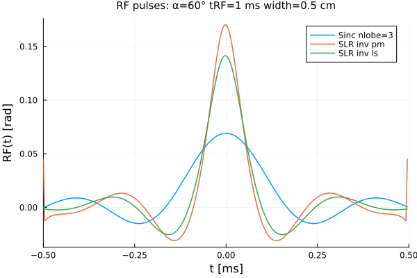
pulse7 = pulse0 * (π / α_rad) # scaled sinc for comparison

plot(pulse8)

prf8 = plot(t, [pulse7 pulse8 pulse9],
  label = [label0 label8 label9],
  xaxis = ("t [ms]", (-1,1) .* (tRF_ms/2), ),
  yaxis = ("RF(t) [rad]", ),
  title = "RF pulses: α=$(α_deg)° tRF=$tRF_ms ms width=$slice_width cm",
)

prompt()

Inversion profiles

rf7, _ = rf_slice(tRF_ms ; nlobe, α_rad = π, Δt_ms, slice_width)
wave8 = pulse8 * b1_gauss(1, Δt_ms) # convert to Gauss for RF()
wave9 = pulse9 * b1_gauss(1, Δt_ms)
rf8 = RF(wave8, Δt_ms, 0, rf0.grad)
rf9 = RF(wave9, Δt_ms, 0, rf0.grad);

spins7, signal7 = exciter(rf7)
spins8, signal8 = exciter(rf8)
spins9, signal9 = exciter(rf9);


pp7 = plot_profile(spins7, label0; α_deg = 180, ymin = -1, ytick = -1:1)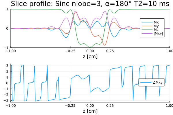

prompt()


pp8 = plot_profile(spins8, label8; α_deg = 180, ymin = -1, ytick = -1:1)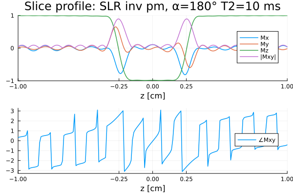

prompt()


pp9 = plot_profile(spins9, label9; α_deg = 180, ymin = -1, ytick = -1:1)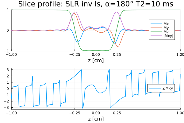

prompt()

This page was generated using Literate.jl.