Use a Custom Sparsifying Transform
The iterative reconstructions can apply the regularization params[:reg] to a transform of the image instead of the image itself, as described in Reconstruction as an Inverse Problem. params[:sparseTrafo] sets this transform: the name "Wavelet", an operator of LinearOperatorCollection.jl or an operator of your own, which LinearOperators.jl helps to build. using MRIReco loads both packages. The example reconstructs a phantom from 48 simulated radial profiles, too few for a good reconstruction without regularization, with ADMM and an
using MRIReco, MRISimulation, Wavelets, FFTW, CairoMakie
using ImageUtils: shepp_logan

N = 128
image = shepp_logan(N)
simParams = Dict{Symbol, Any}()
simParams[:trajName] = "Radial"
simParams[:numProfiles] = 48
simParams[:numSamplingPerProfile] = 2N
acqData = simulation(image, simParams)

params = Dict{Symbol, Any}()
params[:reco] = "standard"
params[:reconSize] = (N, N)
params[:solver] = ADMM
params[:vary_rho] = :balance
params[:iterations] = 50
params[:normalizeReg] = MeasurementBasedNormalization()
params[:reg] = L1Regularization(0.01)
params[:sparseTrafo] = "Wavelet"
imageWavelet = reconstruction(acqData, params)
An Operator of LinearOperatorCollection.jl
The operators of LinearOperatorCollection.jl take the complex element type of the data, ComplexF64 here, and the image size. "Wavelet" is WaveletOp with its default wavelet, Daubechies 2 of Wavelets.jl. The Haar wavelet suits the piecewise constant phantom better:
params[:sparseTrafo] = WaveletOp(ComplexF64; shape = (N, N), wt = wavelet(WT.haar))
imageHaar = reconstruction(acqData, params)
An Operator of Your Own
The operator takes the image as a vector of length prod(params[:reconSize]). A matrix M becomes such an operator with LinearOperator(M); passed as it is, it gives a wrong image or an error (#406). LinearOperator(T, nrows, ncols, symmetric, hermitian, prod!, tprod!, ctprod!) builds one from functions that compute the product and the product with the adjoint in place. As an example, the 2D discrete cosine transform of FFTW.jl gives the same result as DCTOp of LinearOperatorCollection.jl:
function dctOperator(N)
    prod!(res, x) = (res .= vec(dct(reshape(x, N, N))))
    ctprod!(res, y) = (res .= vec(idct(reshape(y, N, N))))
    return LinearOperator(ComplexF64, N * N, N * N, false, false, prod!, nothing, ctprod!)
end

params[:sparseTrafo] = dctOperator(N)
imageDCT = reconstruction(acqData, params)
params[:sparseTrafo] = DCTOp(ComplexF64; shape = (N, N))
reconstruction(acqData, params) ≈ imageDCTtrueTransforms That Are Not Orthonormal
How MRIReco.jl combines the regularization term with the transform depends on the solver. ADMM, which this guide uses, and SplitBregman take the transform separately: they introduce a separate variable for the transformed image and apply the proximal map of the term to it, so they work with any linear transform. FISTA, POGM and OptISTA get the term and the transform combined in a TransformedRegularization of RegularizedLeastSquares.jl, whose proximal map applies the proximal map of the term to the transform coefficients and transforms the result back with the adjoint. This is correct for orthonormal transforms, whose adjoint is their inverse, such as the wavelets and the DCT above, but not for others. With the finite differences of GradientOp, the
params[:sparseTrafo] = GradientOp(ComplexF64; shape = (N, N))
imageGradient = reconstruction(acqData, params)
params[:solver] = FISTA
imageGradientFISTA = reconstruction(acqData, params)
params[:solver] = ADMM
maximum(abs, imageGradient), maximum(abs, imageGradientFISTA)
(0.9998719594522888, 5.9440162796006004e51)The regularization term TVRegularization computes the same total variation with its own proximal map and needs no transform. For ADMM and SplitBregman, their docstrings in RegularizedLeastSquares.jl recommend the GradientOp instead; here both give almost the same image. As in Iterative Reconstruction, TVRegularization gets more inner iterations than by default:
delete!(params, :sparseTrafo)
params[:reg] = TVRegularization(0.01, shape = (N, N), iterationsTV = 50)
imageTV = reconstruction(acqData, params)
The figure compares the five reconstructions by the normalized root mean squared deviation from the phantom. Since the phantom is piecewise constant, the Haar wavelet and the finite differences represent it with few coefficients, and the cosines of the DCT with many, so that the DCT does not improve this reconstruction:
deviation(x) = round(nrmsd(image, abs.(x[:, :, 1, 1, 1, 1])), sigdigits = 2)
images = [imageWavelet => "Daubechies 2", imageHaar => "Haar", imageDCT => "DCT",
          imageGradient => "Finite differences", imageTV => "Total variation"]
fig = Figure(size = (1000, 260))
for (i, (x, title)) in enumerate(images)
    ax = Axis(fig[1, i], title = "$title\nNRMSD $(deviation(x))", aspect = DataAspect(), yreversed = true)
    heatmap!(ax, abs.(x[:, :, 1, 1, 1, 1])', colormap = :grays)
    hidedecorations!(ax)
end
fig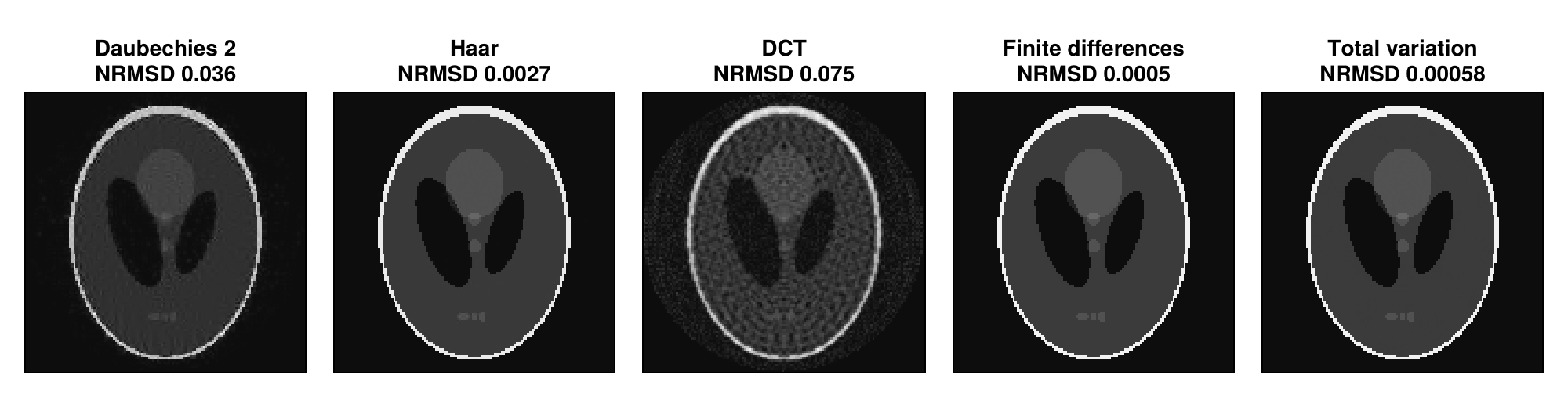
This page was generated using Literate.jl.