Multi-Coil Reconstruction
Each receive coil is most sensitive to the tissue close to it, so the coils see the object with different weightings. These differences carry spatial information, which parallel imaging uses to reconstruct images from undersampled data. This tutorial undersamples the knee data from Direct Reconstruction, estimates the coil sensitivities and reconstructs a single image from the data of all eight coils with the reconstruction type "multiCoil". Finally, it adds a regularization that combines parallel imaging with compressed sensing.
Besides MRIReco, the tutorial needs MRIFiles to read the data, MRISampling to undersample it, MRICoilSensitivities to estimate the coil sensitivities and CairoMakie for the plots. We use the same plotting function as in Direct Reconstruction.
using MRIReco, MRIFiles, MRISampling, MRICoilSensitivities, CairoMakie

function showimages(images, titles; columns = length(images))
    fig = Figure(size = (300 * columns, 310 * cld(length(images), columns)))
    for (i, (image, title)) in enumerate(zip(images, titles))
        ax = Axis(fig[fldmod1(i, columns)...], title = title,
                  aspect = DataAspect(), yreversed = true)
        heatmap!(ax, image', colormap = :grays)
        hidedecorations!(ax)
    end
    return fig
end
Loading the Data
The knee data is fully sampled. Its direct reconstruction, with the coil images combined by the root sum of squares, serves as the reference:
using Pkg.Artifacts
artifacts = joinpath(pkgdir(MRIReco), "docs", "Artifacts.toml")
datadir = ensure_artifact_installed("MRIRecoDocsData", artifacts; io = devnull)
filename = joinpath(datadir, "knee_3dFSE_slice170.h5")
acqData = AcquisitionData(ISMRMRDFile(filename))

params = Dict{Symbol, Any}()
params[:reco] = "direct"
params[:reconSize] = (320, 320)
rootSumOfSquares(images) = sqrt.(sum(abs2, images, dims = 5))[:, :, 1, 1, 1, 1]
referenceImage = rootSumOfSquares(reconstruction(acqData, params))
Undersampling
We keep a quarter of the profiles. sample_kspace chooses them by Poisson-disk sampling and, with calsize = 30, always includes the 30 profiles in the center of k-space. These profiles form a fully sampled calibration region, from which we estimate the coil sensitivities below. The seed makes the random choice reproducible:
acqDataSub = sample_kspace(acqData, 4.0, "poisson", calsize = 30, seed = 1234)

samplingMask = zeros(320, 320)
samplingMask[acqDataSub.subsampleIndices[1]] .= 1
The direct reconstruction of the undersampled data is blurred and shows vertical stripes, because profiles are missing along the horizontal direction. We measure the deviation from the reference with nrmsd, the normalized root mean squared deviation:
directImage = rootSumOfSquares(reconstruction(acqDataSub, params))
deviation(image) = round(nrmsd(referenceImage, image), sigdigits = 2)
showimages([referenceImage, samplingMask, directImage],
           ["Fully sampled", "Sampling mask",
            "Direct, NRMSD $(deviation(directImage))"])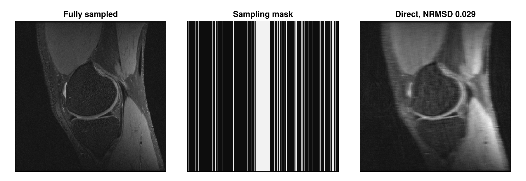
Coil Sensitivities
The reconstruction type "multiCoil" describes the data
where espirit uses the calibration region for this; its second and third arguments are the kernel size and the size of the calibration region. It can also set the sensitivities to zero in voxels without signal. In this slice, the default threshold does this only for some patches of the background, so we turn it off with eigThresh_2 = 0:
sensitivities = espirit(acqDataSub, (6, 6), 30, eigThresh_2 = 0)
size(sensitivities)
(320, 320, 1, 8)The dimensions are x, y, z and coils. Inside the knee, the sensitivities vary smoothly, and the coils are most sensitive in different regions. Outside the knee, where there is no signal, they are not meaningful:
showimages([abs.(sensitivities[:, :, 1, c]) for c in 1:8],
           ["Coil $c" for c in 1:8], columns = 4)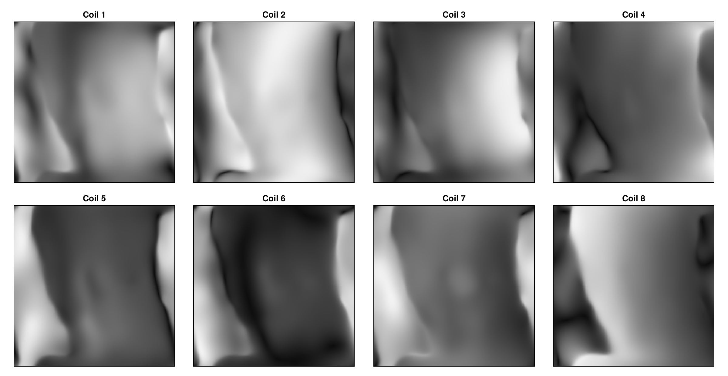
SENSE Reconstruction
From the data of all coils, "multiCoil" reconstructs a single image by solving
Solving this problem with the conjugate gradient method is known as CG-SENSE. We pass the sensitivities as params[:senseMaps] and, as in Iterative Reconstruction, use CGNR with a small MeasurementBasedNormalization, λ is scaled with the magnitude of the data:
params = Dict{Symbol, Any}()
params[:reco] = "multiCoil"
params[:reconSize] = (320, 320)
params[:senseMaps] = sensitivities
params[:solver] = CGNR
params[:reg] = L2Regularization(1e-3)
params[:normalizeReg] = MeasurementBasedNormalization()
params[:iterations] = 10
imageSENSE = abs.(reconstruction(acqDataSub, params)[:, :, 1, 1, 1, 1])
showimages([referenceImage, directImage, imageSENSE],
           ["Fully sampled", "Direct, NRMSD $(deviation(directImage))",
            "CG-SENSE, NRMSD $(deviation(imageSENSE))"])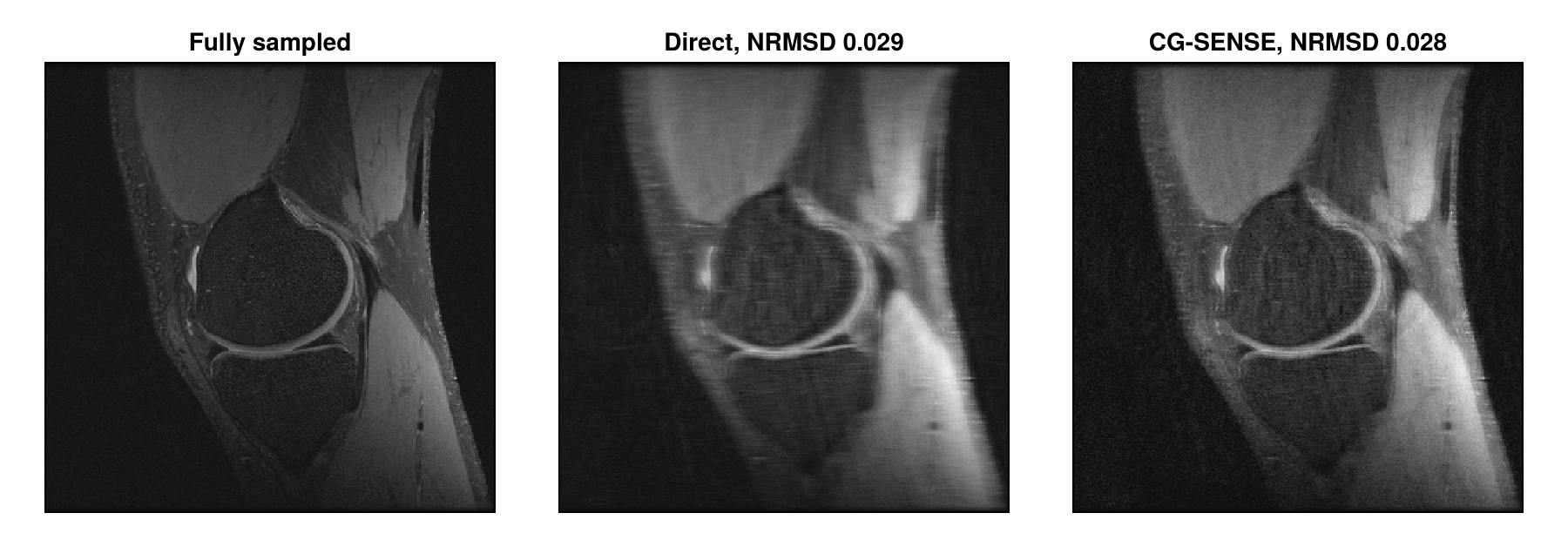
The result is a single image instead of eight coil images. It is sharper than the direct reconstruction, but at this reduction factor, the sensitivities do not suffice to remove all stripes.
Compressed Sensing
MR images can be approximated well by a few large coefficients of a wavelet transform params[:sparseTrafo] = "Wavelet", the
params[:solver] = ADMM
params[:reg] = L1Regularization(0.2)
params[:sparseTrafo] = "Wavelet"
params[:iterations] = 30
imageWavelet = abs.(reconstruction(acqDataSub, params)[:, :, 1, 1, 1, 1])
showimages([referenceImage, imageSENSE, imageWavelet],
           ["Fully sampled", "CG-SENSE, NRMSD $(deviation(imageSENSE))",
            "ℓ1-wavelet, NRMSD $(deviation(imageWavelet))"])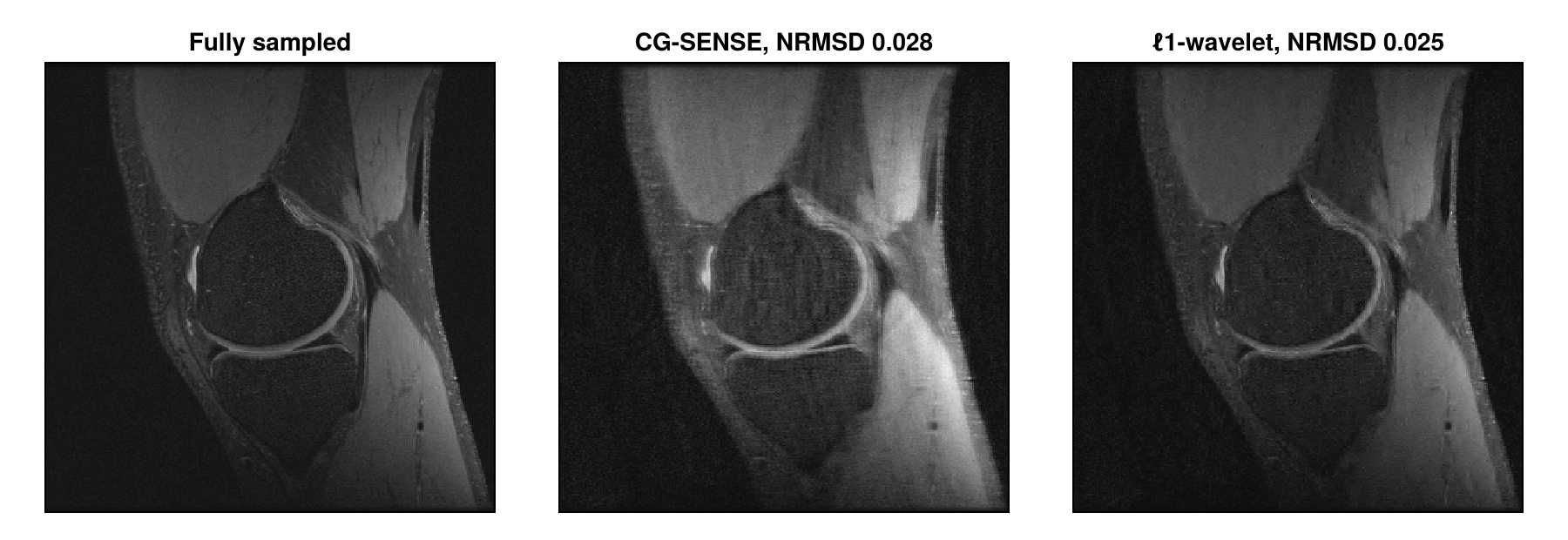
The wavelet regularization reduces the remaining stripes. The differences are easier to see in a detail of the joint:
detail = (100:260, 80:240)
images = [referenceImage, directImage, imageSENSE, imageWavelet]
showimages([image[detail...] for image in images],
           ["Fully sampled", "Direct", "CG-SENSE", "ℓ1-wavelet"])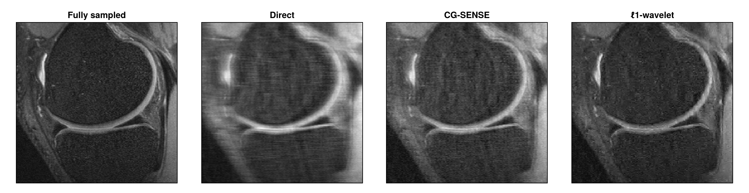
Next Steps
Iterative Reconstruction shows how the weight λ changes the result.
Signal Model and Encoding Operators explains how the coil sensitivities enter the encoding operator.
The RegularizedLeastSquares.jl documentation describes the available solvers and regularization terms.
Estimate Coil Sensitivities with ESPIRiT shows how to choose the calibration region and mask voxels without signal, Compress Multi-Coil Data how to reduce the number of coils, and Run a Reconstruction on the GPU how to move the reconstruction to a GPU.
Reconstruction Parameters lists the keys of the parameter dictionary, and the API reference describes
reconstruction,espiritandsample_kspace.
This page was generated using Literate.jl.