Getting Started
Installation
MRIReco.jl requires Julia 1.10 or newer. Install the main package with
using Pkg
Pkg.add("MRIReco")
using MRIReco also loads MRIBase, MRIOperators, RegularizedLeastSquares.jl, which provides the solvers, and AbstractImageReconstruction.jl, which provides the functions for reconstruction plans. The other packages are installed in the same way when you need them, for example Pkg.add("MRIFiles") to read raw data files. The examples in this documentation also use CairoMakie for plots and ImageUtils for test images.
Development Version
The development documentation describes the master branch, which can contain changes that are not released yet. To use master, add the package and the packages of this repository that it depends on, each with rev = "master". Otherwise Pkg takes these dependencies from the registry, and their released versions may not work with master. For MRIReco, which depends on MRIBase and MRIOperators:
using Pkg
Pkg.add([PackageSpec(name = "MRIBase", rev = "master"),
         PackageSpec(name = "MRIOperators", rev = "master"),
         PackageSpec(name = "MRIReco", rev = "master")])
For other packages, such as MRIFiles or MRISimulation, the table of packages on the Home page lists the packages of this repository that they depend on. Pkg.update() moves the packages to the newest commit of master, and Pkg.free(["MRIBase", "MRIOperators", "MRIReco"]) returns them to their released versions. To work on the packages themselves, follow the development setup of the contributing guide.
A First Reconstruction
This example simulates k-space data of a Shepp-Logan phantom along a radial trajectory and reconstructs an image from it. Besides MRIReco it needs MRISimulation, ImageUtils and CairoMakie.
using MRIReco, MRISimulation, CairoMakie
using ImageUtils: shepp_logan

N = 256
phantom = shepp_logan(N)

params = Dict{Symbol, Any}()
params[:simulation] = "fast"
params[:trajName] = "Radial"
params[:numProfiles] = floor(Int64, pi/2 * N)
params[:numSamplingPerProfile] = 2N
acqData = simulation(phantom, params)
acqData is an AcquisitionData object that holds the simulated k-space data together with the trajectory. A direct reconstruction applies the adjoint of the Fourier encoding to the density-compensated data:
params = Dict{Symbol, Any}()
params[:reco] = "direct"
params[:reconSize] = (N, N)
image = reconstruction(acqData, params)
size(image)
(256, 256, 1, 1, 1, 1)The reconstructed image always has six dimensions: x, y, z, echoes, coils and repetitions. Here only the first two have more than one entry:
images = [phantom, abs.(image[:, :, 1, 1, 1, 1])]
titles = ["Phantom", "Reconstruction"]
fig = Figure(size = (700, 350))
for i in 1:2
    ax = Axis(fig[1, i], aspect = DataAspect(), yreversed = true, title = titles[i])
    heatmap!(ax, images[i]', colormap = :grays)
    hidedecorations!(ax)
end
fig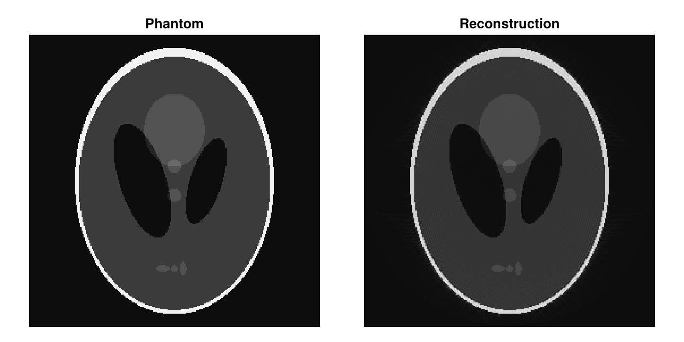
Next Steps
The tutorials walk through complete reconstructions step by step, starting with Direct Reconstruction and Iterative Reconstruction.
The how-to guides show how to solve specific tasks, such as simulating k-space data, loading and saving raw data, binning profiles, extracting Cartesian k-space data or running a reconstruction on the GPU.
The explanations describe the design of the packages and the concepts behind them, for example the data model and reconstruction as an inverse problem.
Reconstruction Parameters lists the keys that
reconstructiontakes, and Configure a Reconstruction with Plans shows the reconstruction plans that it fills with them. The API reference describes the functions and types of each package.