Iterative Reconstruction
Acquiring fewer k-space samples shortens the scan, but a direct reconstruction of undersampled data shows artifacts. An iterative reconstruction instead searches for the image that agrees best with the measured samples, and it can use prior knowledge about the image. This tutorial undersamples single-coil data and compares the direct reconstruction with the iterative reconstruction type "standard".
Besides MRIReco, the tutorial needs MRIFiles to read the data, MRISampling to undersample it and CairoMakie for the plots. We use the same plotting function as in Direct Reconstruction.
using MRIReco, MRIFiles, MRISampling, CairoMakie

function showimages(images, titles; columns = length(images))
    fig = Figure(size = (300 * columns, 310 * cld(length(images), columns)))
    for (i, (image, title)) in enumerate(zip(images, titles))
        ax = Axis(fig[fldmod1(i, columns)...], title = title,
                  aspect = DataAspect(), yreversed = true)
        heatmap!(ax, image', colormap = :grays)
        hidedecorations!(ax)
    end
    return fig
end
Loading the Data
The data is a simulated single-coil dataset of a brain image with 256 × 256 pixels, fully sampled on a Cartesian grid. The file belongs to the documentation data, which is downloaded as in Direct Reconstruction. The direct reconstruction of the fully sampled data serves as the reference. Of the six dimensions of the reconstructed image, we keep x and y and take the magnitude:
using Pkg.Artifacts
artifacts = joinpath(pkgdir(MRIReco), "docs", "Artifacts.toml")
datadir = ensure_artifact_installed("MRIRecoDocsData", artifacts; io = devnull)
filename = joinpath(datadir, "acqDataBrainSim100.h5")
acqData = AcquisitionData(ISMRMRDFile(filename))

params = Dict{Symbol, Any}()
params[:reco] = "direct"
params[:reconSize] = (256, 256)
referenceImage = abs.(reconstruction(acqData, params)[:, :, 1, 1, 1, 1])
Undersampling
To simulate an acquisition that is three times faster, sample_kspace keeps about a third of the profiles. They are chosen by variable-density Poisson-disk sampling, which samples the center of k-space more densely than the outer parts, and the seed makes this random choice reproducible. The result is a new AcquisitionData object that stores the indices of the kept samples in subsampleIndices:
acqDataSub = sample_kspace(acqData, 3.0, "vdPoisson", seed = 1234)

samplingMask = zeros(256, 256)
samplingMask[acqDataSub.subsampleIndices[1]] .= 1
The direct reconstruction treats the missing samples as zeros, which causes aliasing artifacts. We measure the deviation from the reference with nrmsd, the normalized root mean squared deviation:
directImage = abs.(reconstruction(acqDataSub, params)[:, :, 1, 1, 1, 1])
deviation(image) = round(nrmsd(referenceImage, image), sigdigits = 2)
showimages([referenceImage, samplingMask, directImage],
           ["Fully sampled", "Sampling mask",
            "Direct, NRMSD $(deviation(directImage))"])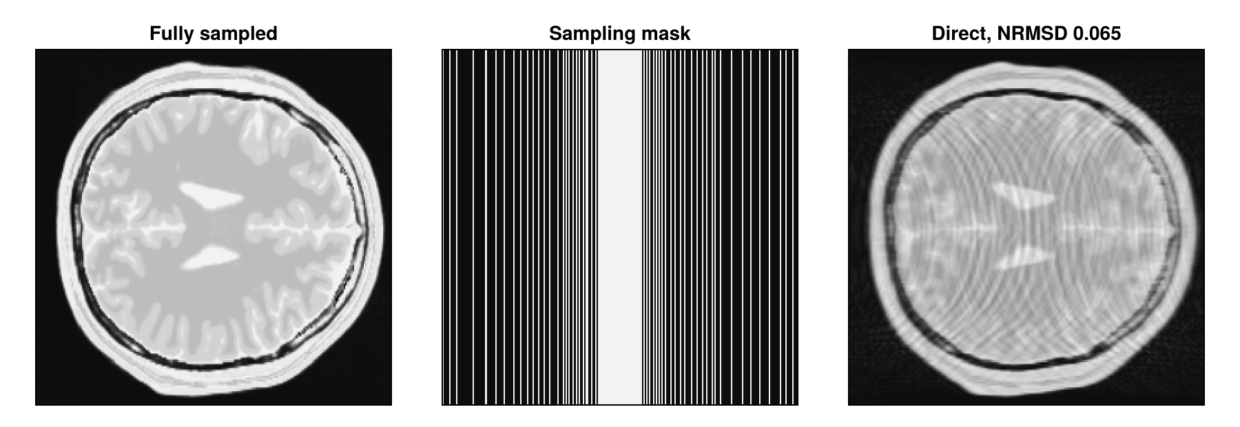
Iterative Reconstruction
The reconstruction type "standard" solves the regularized least-squares problem
where using MRIReco loads.
We first use CGNR, the conjugate gradient method applied to the normal equations, with a small
params = Dict{Symbol, Any}()
params[:reco] = "standard"
params[:reconSize] = (256, 256)
params[:solver] = CGNR
params[:reg] = L2Regularization(1e-3)
params[:iterations] = 20
imageL2 = abs.(reconstruction(acqDataSub, params)[:, :, 1, 1, 1, 1])
showimages([referenceImage, directImage, imageL2],
           ["Fully sampled", "Direct, NRMSD $(deviation(directImage))",
            "CGNR and ℓ2, NRMSD $(deviation(imageL2))"])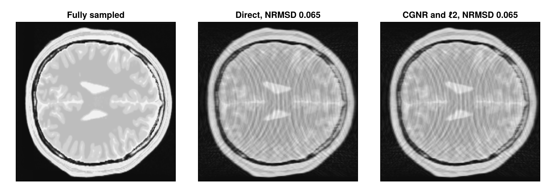
The result is practically the same as the direct reconstruction. The data term only involves the measured samples, and the
Total Variation
Total variation (TV) regularization, which penalizes rho with vary_rho = :balance and use more inner iterations for the TV term than by default, iterationsTV = 50. With MeasurementBasedNormalization, λ is scaled with the magnitude of the data, so that the same value works for data of different scale:
params[:solver] = ADMM
params[:vary_rho] = :balance
params[:reg] = TVRegularization(0.03, shape = (256, 256), iterationsTV = 50)
params[:normalizeReg] = MeasurementBasedNormalization()
params[:iterations] = 50
imageTV = abs.(reconstruction(acqDataSub, params)[:, :, 1, 1, 1, 1])
showimages([referenceImage, directImage, imageTV],
           ["Fully sampled", "Direct, NRMSD $(deviation(directImage))",
            "TV, NRMSD $(deviation(imageTV))"])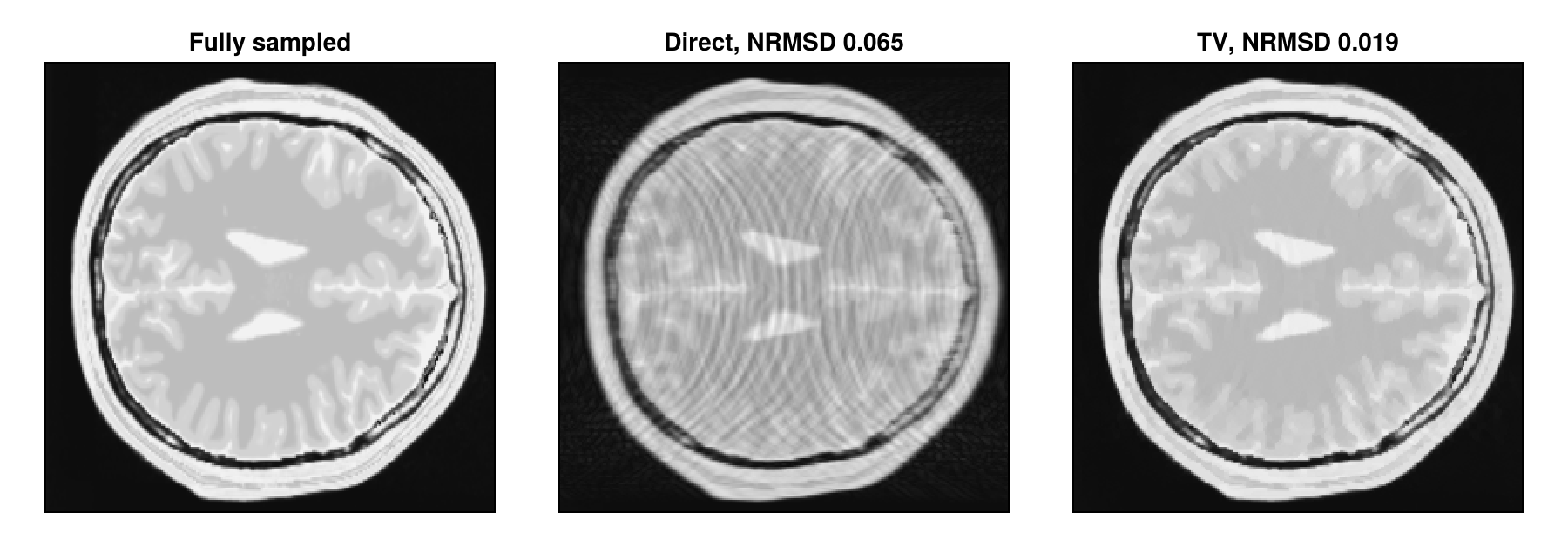
The TV reconstruction removes most of the artifacts.
Choosing λ
The weight λ balances the agreement with the measured samples against the regularization. The larger it is, the smoother the image becomes, and if it is too large, details are lost:
lambdas = [0.003, 0.03, 0.3]
images = map(lambdas) do λ
    params[:reg] = TVRegularization(λ, shape = (256, 256), iterationsTV = 50)
    abs.(reconstruction(acqDataSub, params)[:, :, 1, 1, 1, 1])
end
showimages(images, ["λ = $λ, NRMSD $(deviation(image))"
                    for (λ, image) in zip(lambdas, images)])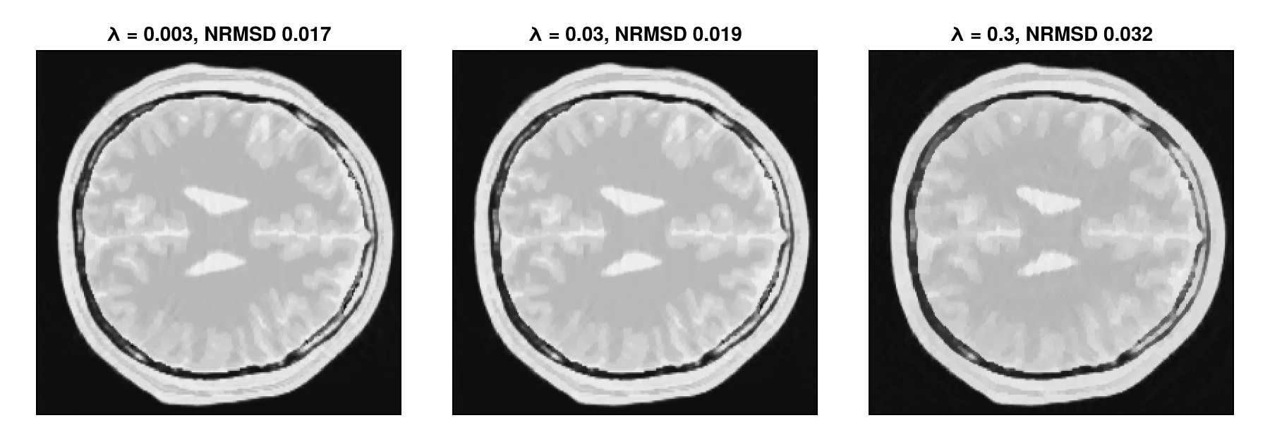
Because the simulated data contains no noise, even λ = 0.003 gives an image similar to λ = 0.03, while λ = 0.3 loses details. Measured data contains noise, and a small λ leaves more of it in the image. The best value depends on the data, its noise and the undersampling, so it is usually found by comparing several reconstructions.
Next Steps
Reconstruction as an Inverse Problem explains the problem in more detail, with the weighting of the samples and the normalization of λ, and the RegularizedLeastSquares.jl documentation describes the available solvers and regularization terms.
With several coils,
"standard"reconstructs the image of each coil separately. Multi-Coil Reconstruction shows how the reconstruction type"multiCoil"uses the coil sensitivities to reconstruct a single image from all coils.With several echoes,
"standard"reconstructs each echo on its own. Multi-Echo Reconstruction shows how the reconstruction type"multiEcho"reconstructs them jointly.Undersample k-Space shows how to choose and reproduce a sampling pattern, and Use a Custom Sparsifying Transform how to apply the regularization to other transforms of the image.
Reconstruction Parameters lists the keys of the parameter dictionary, and the API reference describes
reconstructionandsample_kspace.
This page was generated using Literate.jl.