Use a Plug-and-Play Prior
A plug-and-play (PnP) method replaces the proximal map of the regularization term in an iterative reconstruction by an image denoiser (Venkatakrishnan et al., 2013). This way, any denoising algorithm can serve as the prior, including one without a known cost function such as a trained neural network, with which PnP outperformed compressed sensing in the MRI experiments of Ahmad et al. (2020). RegularizedLeastSquares.jl provides the regularization term PnPRegularization (see its how-to), which params[:reg] takes like any other term. This guide shows how to use a denoiser in reconstruction with the knee data, sampling and coil sensitivities of Multi-Coil Reconstruction:
using MRIReco, MRIFiles, MRISampling, MRICoilSensitivities, CairoMakie
using Pkg.Artifacts

artifacts = joinpath(pkgdir(MRIReco), "docs", "Artifacts.toml")
datadir = ensure_artifact_installed("MRIRecoDocsData", artifacts; io = devnull)
acqData = AcquisitionData(ISMRMRDFile(joinpath(datadir, "knee_3dFSE_slice170.h5")))
rootSumOfSquares(images) = sqrt.(sum(abs2, images, dims = 5))[:, :, 1, 1, 1, 1]
referenceImage = rootSumOfSquares(
    reconstruction(acqData, Dict{Symbol, Any}(:reco => "direct", :reconSize => (320, 320))))
acqDataSub = sample_kspace(acqData, 4.0, "poisson", calsize = 30, seed = 1234)
sensitivities = espirit(acqDataSub, (6, 6), 30, eigThresh_2 = 0)
The Denoiser
The denoiser is a function of one array. PnPRegularization calls it with an array of the size shape, separately for the real and the imaginary part of the image, each scaled to the interval [0, 1], and expects a new array of the same size back. It must not change its argument, which is why the denoiser below works on a copy. The array has the precision of the data, here Float32. With ignoreIm = true, PnPRegularization denoises the real part only, which real-valued images need, since the scaling would turn their zero imaginary part into NaN. This guide uses a denoiser that comes with RegularizedLeastSquares.jl and needs no further package, the proximal map of the total variation, whose weight sets how strongly it smooths:
function tvDenoiser(x)
    y = vec(copy(x))
    prox!(TVRegularization(0.01f0; shape = size(x)), y)
    return reshape(y, size(x))
end
Solver Settings
The weight of PnPRegularization, its first argument, works differently from the weight λ of the other terms. In each iteration, the term replaces its input params[:rho], so a weight of params[:vary_rho] = :PnP, ADMM doubles params[:vary_rho] = :balance can also halve
shape is a vector, so the guide converts the tuple params[:reconSize]. The weight must not be scaled with the data, so the guide sets params[:normalizeReg] explicitly to its default, NoNormalization():
params = Dict{Symbol, Any}()
params[:reco] = "multiCoil"
params[:reconSize] = (320, 320)
params[:senseMaps] = sensitivities
params[:solver] = ADMM
params[:rho] = 0.1
params[:vary_rho] = :PnP
params[:normalizeReg] = NoNormalization()
params[:reg] = PnPRegularization(2 * params[:rho]; model = tvDenoiser,
                                 shape = collect(params[:reconSize]))
params[:iterations] = 30
imagePnP = abs.(reconstruction(acqDataSub, params)[:, :, 1, 1, 1, 1])
FISTA takes params[:rho] as its step size and passes the weight multiplied by it, so a weight of params[:rho] as their step size, but multiply the weight by larger factors that change from iteration to iteration. With POGM, the factor stays below
Comparison
For comparison, the guide computes the CG-SENSE and the
paramsCS = Dict{Symbol, Any}(:reco => "multiCoil", :reconSize => (320, 320),
                             :senseMaps => sensitivities,
                             :normalizeReg => MeasurementBasedNormalization())
paramsCS[:solver] = CGNR
paramsCS[:reg] = L2Regularization(1e-3)
paramsCS[:iterations] = 10
imageSENSE = abs.(reconstruction(acqDataSub, paramsCS)[:, :, 1, 1, 1, 1])
paramsCS[:solver] = ADMM
paramsCS[:reg] = L1Regularization(0.2)
paramsCS[:sparseTrafo] = "Wavelet"
paramsCS[:iterations] = 30
imageWavelet = abs.(reconstruction(acqDataSub, paramsCS)[:, :, 1, 1, 1, 1])
The figure shows a detail of the joint and, in the titles, the normalized root mean squared deviation of the whole image from the fully sampled one. Like the
deviation(image) = round(nrmsd(referenceImage, image), sigdigits = 2)
detail = (100:260, 80:240)
images = [referenceImage => "Fully sampled",
          imageSENSE => "CG-SENSE, NRMSD $(deviation(imageSENSE))",
          imageWavelet => "ℓ1-wavelet, NRMSD $(deviation(imageWavelet))",
          imagePnP => "PnP with TV, NRMSD $(deviation(imagePnP))"]
fig = Figure(size = (1200, 330))
for (i, (image, title)) in enumerate(images)
    ax = Axis(fig[1, i], title = title, aspect = DataAspect(), yreversed = true)
    heatmap!(ax, image[detail...]', colormap = :grays)
    hidedecorations!(ax)
end
fig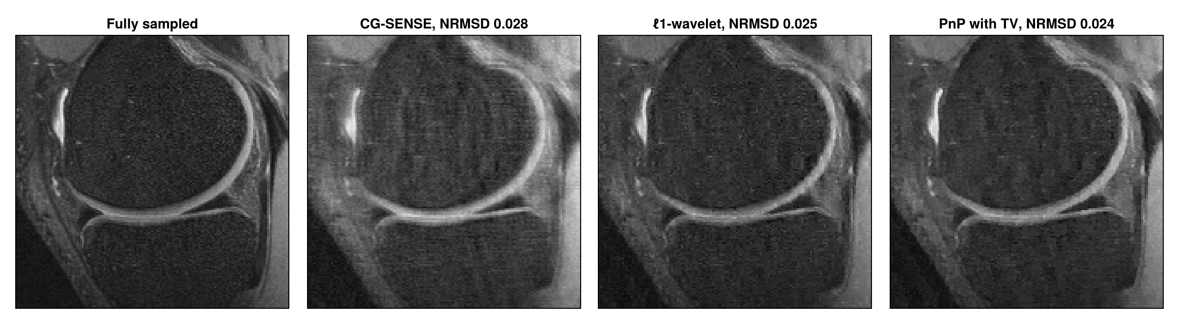
A Trained Network
A trained network takes the place of tvDenoiser as model; PnPRegularization passes the real and the imaginary part one at a time, a network that takes both parts together as two channels, as in Ahmad et al. (2020), does not fit it. For a Flux.jl model net that expects one channel and a batch dimension, the denoiser could be:
denoiser(x) = reshape(net(reshape(x, size(x)..., 1, 1)), size(x))If the network was trained on a scaling other than [0, 1], the keyword input_transform of PnPRegularization selects it, for example input_transform = RegularizedLeastSquares.ZTransform for zero mean and unit standard deviation.
Limits
For a denoiser that is not the proximal map of a regularization term, the iterations are not guaranteed to converge. Chan et al. (2017) prove fixed-point convergence with their adaptive
for bounded denoisers, and Kamilov et al. (2023) review further conditions, which trained networks can be made to satisfy. A denoiser that smooths too little lets the result approach the one of the same solver without regularization.
MeasurementBasedNormalization, which the-wavelet reconstruction above uses, also scales the weight of PnPRegularization, here by about 174. The passed weight is then set to 1 with warnings in every iteration, and the result is worse than without the normalization.The denoiser,
params[:rho]and the weight of this guide are chosen for ADMM. With FISTA, the same denoiser applied fully gives a worse result than CG-SENSE, so they have to be chosen again for another solver.
This page was generated using Literate.jl.